3D Gaussian splatting is the emerging rendering technique that is overtaking NeRFs. Since it is centered around point primitives, it is more compatible with traditional graphics pipelines that already support point rendering.

Gaussian splats essentially enhance the concept of point rendering by converting the point primitive into a 3D ellipsoid, which is then projected into 2D during the rendering process.. This concept was initially described in 2002 [3], but the technique of extending Structure from Motion scans in this way was only detailed more recently [1].

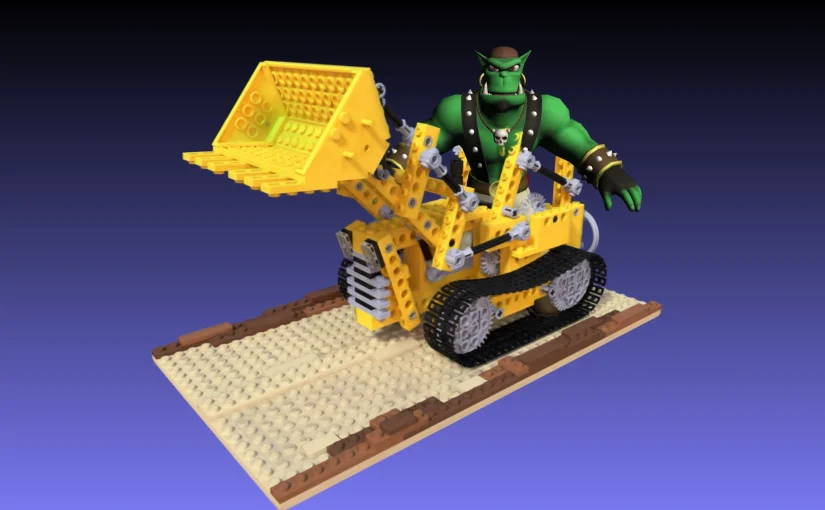
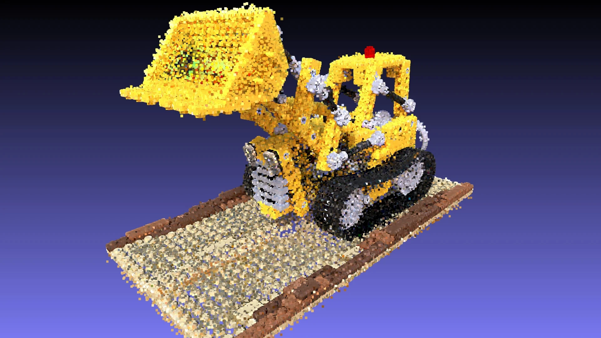
In this post, I explore how to integrate Gaussian splats into the traditional graphics pipeline. This allows them to be used alongside triangle-based primitives and interact with them through the depth buffer for occlusion (see header image). This approach also simplifies deployment by eliminating the need for CUDA.

Storage

The original implementation uses .ply files as their checkpoint format, focusing on maintaining training-relevant data structures at the expense of storage efficiency, leading to increased file sizes.

For example, it stores the covariance as scaling and a rotation quaternion, necessitating reconstruction during rendering. A more efficient approach would be to leverage orthogonality, storing only the diagonal and upper triangular vectors, thereby eliminating reconstruction and reducing storage requirements.

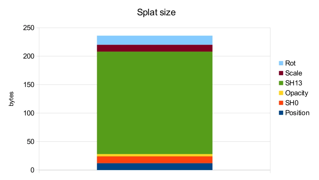
Further analysis of the storage usage for each attribute shows that the spherical harmonics of orders 1-3 are the main contributors to the file size. However, according to the ablation study in the original publication [1], these harmonics only lead to a modest PSNR improvement of 0.5.

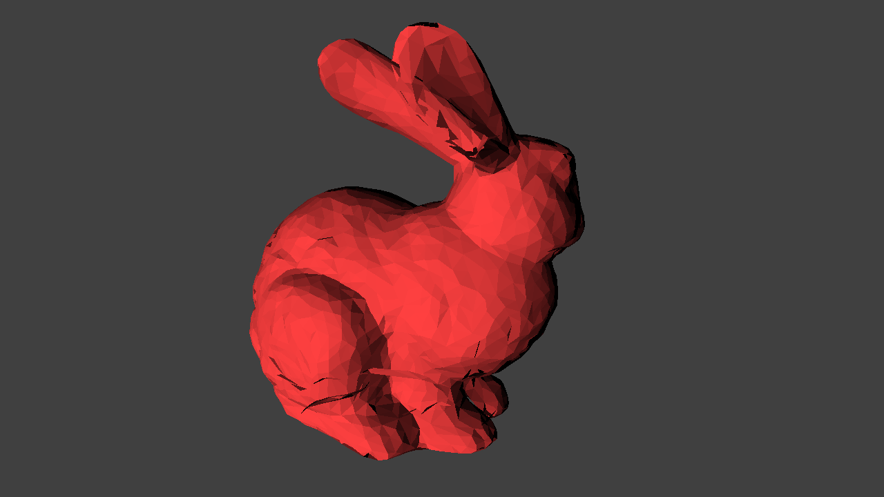
Therefore, the most straightforward way to decrease storage is by discarding the higher-order spherical harmonics. Additionally, the level 0 spherical harmonics can be converted into a diffuse color and merged with opacity to form a single RGBA value. These simple yet effective methods were implemented in one of the early WebGL implementations, resulting in the .splat format. As an added benefit, this format can be easily interpreted by viewers unaware of Gaussian splats as a simple colored point cloud:

By directly storing the covariance as previously mentioned we can reduce the precision from float32 to float16, thereby halving the storage needed for that data. Furthermore, since most splats have limited spatial extents, we can also utilize float16 for position data, yielding additional storage savings.

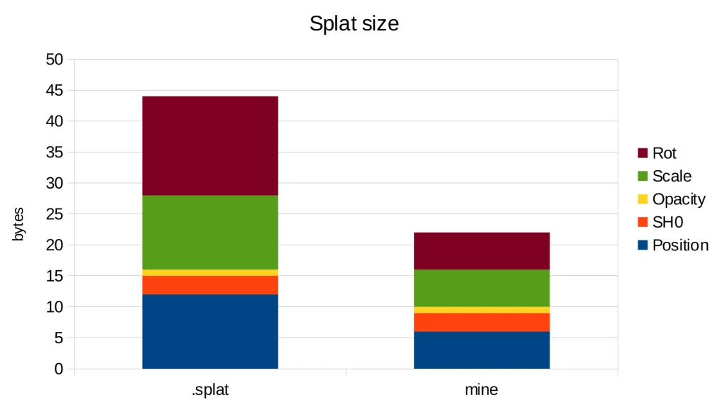
With these changes, we achieve a storage requirement of 22 bytes per splat, in contrast to the 44 bytes needed by the .splat format and 236 bytes in the original implementation. Thus, we have attained a 10x reduction in storage compared to the original implementation simply by using more suitable data types.

Blending

The image formation model presented in the original paper [1] is similar to the NeRF rendering, as it is compared to it. This involves casting a ray and observing its intersection with the splats, which leads to front-to-back blending. This is precisely the approach taken by the provided CUDA implementation.

Blending remains a component of the fixed-function unit within the graphics pipeline, which can be set up for front-to-back blending [2] by using the factors (one_minus_dest_alpha, one) and by multiplying color and alpha in the shader as color.rgb * color.a. This results in the following equation:

\begin{aligned}C_{dst} &= (1 - \alpha_{dst}) \cdot \alpha_{src} C_{src} &+ C_{dst}\\ \alpha_{dst} &= (1 - \alpha_{dst})\cdot\alpha_{src} &+ \alpha_{dst}\end{aligned}

However, this method requires the framebuffer alpha value to be zero before rendering the splats, which is not typically the case as any previous render pass could have written an arbitrary alpha value.

A simple solution is to switch to back-to-front sorting and use the standard alpha blending factors (src_alpha, one_minus_src_alpha) for the following blending equation:

C_{dst} = \alpha_{src} \cdot C_{src} + (1 - \alpha_{src}) \cdot C_{dst}

This allows us to regard Gaussian splats as a special type of particles that can be rendered together with other transparent elements within a scene.

References

1. Kerbl, Bernhard, et al. “3d gaussian splatting for real-time radiance field rendering.” ACM Transactions on Graphics 42.4 (2023): 1-14.
2. Green, Simon. “Volumetric particle shadows.” NVIDIA Developer Zone (2008).
3. Zwicker, Matthias, et al. “EWA splatting.” IEEE Transactions on Visualization and Computer Graphics 8.3 (2002): 223-238.

This question often pops up, when you need a random direction vector to place things in 3D or you want to do a particle simulation.

We recall that a 3D unit-sphere (and hence a direction) is parametrized only by two variables; elevation \theta \in [0; \pi] and azimuth \varphi \in [0; 2\,\pi] which can be converted to Cartesian coordinates as

\begin{aligned} x &= \sin\theta \, \cos\varphi \\ y &= \sin\theta \, \sin\varphi \\ z &= \cos\theta \end{aligned}

If one takes the easy way and uniformly samples this parametrization in numpy like

phi = np.random.rand() * 2 * np.pi
theta = np.random.rand() * np.pi

One (i.e. you as you are reading this) ends with something like this:

While the 2D surface of polar coordinates uniformly sampled (left), we observe a bias of sampling density towards the poles when projecting to the Cartesian coordinates (right).
The issue is that the cos mapping of the elevation has an uneven step size in Cartesian space, as you can easily verify: cos^{'}(x) = sin(x).

The solution is to simply sample the elevation in the Cartesian space instead of the spherical space – i.e. sampling z \in [-1; 1]. From that we can get back to our elevation as \theta = \arccos z:

z = 1 - np.random.rand() * 2 # convert rand() range 0..1 to -1..1
theta = np.arccos(z)

As desired, this compensates the spherical coordinates such that we end up with uniform sampling in the Cartesian space:

Custom opening angle

If you want to further restrict the opening angle instead of sampling the full sphere you can also easily extend the above. Here, you must re-map the cos values from [1; -1] to [0; 2] as

cart_range = -np.cos(angle) + 1 # maximal range in cartesian coords
z = 1 - np.random.rand() * cart_range
theta = np.arccos(z)

Optimized computation

If you do not actually need the parameters \theta, \varphi, you can spare some trigonometric functions by using \sin \theta = \sqrt { 1 - z^2} as

\begin{aligned} x &= \sqrt { 1 - z^2} \, \cos\varphi \\ y &= \sqrt { 1 - z^2} \, \sin\varphi \end{aligned}